“The How of Parameter-Efficient Fine-Tuning with LoRA: Exploring the Inner Workings”

Part 1 delves into the concept and necessity of fine-tuning pre-trained large models for specialized tasks. It introduces the conventional method of fine-tuning, where only the top layers of the model are adjusted, and highlights its limitations, particularly in terms of computational and storage demands. To address these challenges, the article shifts focus to Parameter-Efficient Fine-Tuning (PEFT) methods, specifically the use of adapter modules, as proposed by Houlsby and colleagues. These adapters are small, inserted layers that allow for task-specific training without altering the entire model, significantly reducing computational and storage costs.

The article then explores the concept of a model’s intrinsic dimension, as discussed in works by Li et al. and Aghajanyan et al., suggesting that LLMs can be effectively fine-tuned with a surprisingly small subset of parameters. This leads to the introduction of Low-Rank Adaptation (LoRA), a method that hypothesizes the possibility of decomposing adapters into low-rank matrices for efficient fine-tuning. This is followed by a discussion on principles of low-rank matrix approximation and its application in LoRA.

Set the stage — Data, Model, Library, Pre-training

Huggingface has developed the peft (parameter efficient fine-tuning techniques) library to facilitate the parameter efficient adaptation of pre-trained language models for various downstream applications without fine-tuning all of the model’s parameters. The peft library supports multiple fine-tuning methods one of which is LoRA (Low Rank Adapters) and it can be applied to various model types, not limited to transformers.

There is an abundance of tutorials and blogs discussing how to implement LoRA fine-tuning to Large Language Models (LLMs) such as LLaMa and alike. Grasping the methodology and rationale behind LoRA while applying to large models is challenging because of the inherent complexity of the models. To enhance our understanding, let’s implement LoRA in a multilayer perceptron (MLP) and use it to train a model for a binary classification task and thereby also assess parameter efficiency during the fine-tuning process. In the following sections of this article, we’ll explore select excerpts of code from the accompanying notebook to enhance our understanding.

Let’s create a toy dataset consisting of random data for a classification task.

# Returns a tensor filled with random numbers from a uniform distribution 
# on the interval [0,1).
X = torch.rand((1000, 20)) 

# y is the label with shape (1000, 1) which results in 1 if the 
# sin(sum of elements) in each row is > 0 and 0 otherwise. y is then cast to (torch.int64).
y = (torch.sin(X.sum(1)) > 0).long()

As a model, we use a simple multilayer perceptron (MLP). For demonstration purposes, we use a very large number of hidden units. This is totally an overkill for this task but it helps to demonstrate the advantages of peft. In more realistic settings, models will also be quite large on average, so this is not far-fetched.

print(base_model)
print_trainable_parameters(base_model)

Output:
MLP(
(seq): Sequential(
(0): Linear(in_features=20, out_features=2000, bias=True)
(1): ReLU()
(2): Linear(in_features=2000, out_features=200, bias=True)
(3): ReLU()
(4): Linear(in_features=200, out_features=2, bias=True)
(5): LogSoftmax(dim=-1)
)
)

trainable params: 442602 || all params: 442602 || trainable%: 100.0

There is a little bit of signal in the data, so we should expect that the loss of the model can improve during training.

# Let's train the base model for 20 epochs
train(base_model, optimizer, criterion, train_dataloader, eval_dataloader, epochs=20)

Output:
epoch=0 train_loss_total=0.6282 eval_loss_total=0.5629
epoch=1 train_loss_total=0.5087 eval_loss_total=0.4953
...
epoch=18 train_loss_total=0.1417 eval_loss_total=0.4038
epoch=19 train_loss_total=0.1152 eval_loss_total=0.3991

We achieved an evaluation loss that is better than a random outcome. In fine-tuning exercises, the primary focus is typically on the model’s performance for a specific downstream task. It’s important to note that showcasing performance improvements with LoRA fine-tuning on our current MLP model pre-trained on toy dataset may not be ideal, mainly because its advantages are more pronounced in larger models with clearly defined downstream tasks. Nonetheless, our objective here is to assess how LoRA enhances parameter efficiency and to deepen our understanding of its algorithm. This exploration is particularly relevant because comprehending the implementation of LoRA at code level on large models can be quite challenging.

Fine-tuning with LoRA

Using our model, pre-trained for 20 epochs as a base_model, we’ll apply LoRA using Huggingface’s peft library. Make sure that you have the latest version of peft installed. We already established that we will be injecting few extra set of parameters called adapters in between the layers of the pre-trained based model, focusing on training only these adapters while keeping the base model’s parameters frozen. Where and How to inject the adapters in the base model is still an open question.

Where to inject the adapters?

In the current scenario with a 5-layer MLP, the exact layer for adapter insertion is not particularly critical. However, in larger models, each layer serves a distinct function and contributes differently to learning. For instance, linear layers convey crucial information, unlike layer normalization in a transformer network. To prevent catastrophic forgetting of the original model, adapter modules must be strategically inserted between these impactful layers. Section 7.1 of the LoRA paper¹ conducts experiments to determine which layers can be effectively used for fine-tuning and which ones should remain undisturbed.# Let’s identify the names of the modules, ensuring that we fine-tune
# the appropriate ones with adaptors.
print([(n, type(m)) for n, m in base_model.named_modules()])

Output:
[(”, __main__.MLP),
(‘seq’, torch.nn.modules.container.Sequential),
(‘seq.0’, torch.nn.modules.linear.Linear),
(‘seq.1’, torch.nn.modules.activation.ReLU),
(‘seq.2’, torch.nn.modules.linear.Linear),
(‘seq.3’, torch.nn.modules.activation.ReLU),
(‘seq.4’, torch.nn.modules.linear.Linear),
(‘seq.5’, torch.nn.modules.activation.LogSoftmax)]

How to inject the adapters?

Now we are going to address the ‘how’ part of the question. Let’s say we choose to place adapters for linear layers seq.0 and seq.2 of the base model which we can refer to as ‘Adoptee layers,’ as in this article³. Adapters can be placed either in sequence or in parallel to the adoptee layers. Since adapters are small in size compared to adoptee layers, running it in sequence will be inefficient to work with GPU on two counts – GPU memory wont be fully utilized and GPUs are designed for parallel execution so layers in-sequence will cause time inefficiency.

Authors of LoRA proposed placing adapters in parallel to the adoptee layers. This design keeps the adoptee’s weight matrix and the adapter’s matrix separate throughout the fine-tuning process. Both adoptee and adapter must have the same input and output layer dimension so that parallel connection can be accommodated.

LoRA proposed decomposing the adapter matrix into two low rank matrices (lora_A and lora_B) which will have very small rank. The adapter with lora_A and lora_B is designed such that the output of their product and output of the adoptee layer are compatible. Only lora_A and lora_B are learned for the specific downstream task.

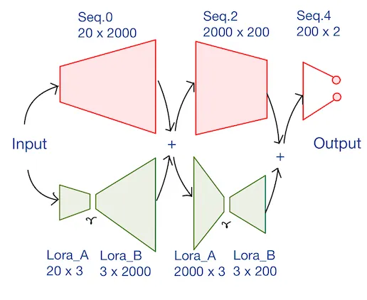
Let’s define the LoRA configuration. We set the LoRA rank to 3 and select the layers seq.0 and seq.2 to be used for LoRA fine-tuning. lora_A and lora_B layers are created across both seq.0 and seq.2layers. Number of parameters in lora_A (20 x 3) + number of parameters in lora_B (3 x 2000) == 6060 is much fewer than the number of parameters in seq.0 (20 x 2000) == 40,000. However, the output dimension of lora_A x lora_Band seq.0 are both equal to 2000, irrespective of the value of r! Both the outputs can now be added and passed to the next module of the network.

Currently, peft allows fine-tuning of Linear, Embedding, Conv2D and Conv1Dlayers in conjunction with LoRA.

config = peft.LoraConfig(    r=3,    target_modules=["seq.0", "seq.2"],)peft_model = peft.get_peft_model(base_model, config)print(peft_model.print_trainable_parameters())Output:trainable params: 12,660 || all params: 455,262 || trainable%: 2.78

We see that only ~2.8% of parameters are actually trainable, which is what we like to see. Now let’s see how detailed architecture of the model with LoRA weights look like:

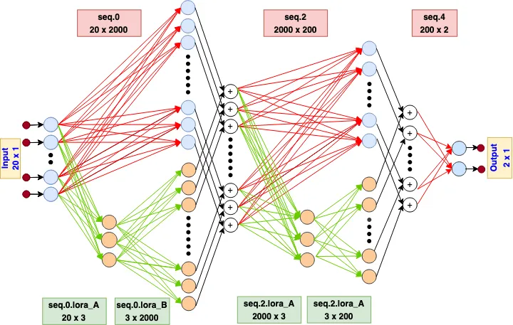
def forward(x):
  seq.0_out = seq.0(x)
  lora_A_out = seq.0.lora_A(x)
  lora_B_out = seq.0.lora_B(lora_A_out)
  lora_B_out = lora_B_out * alpha
  seq.0_lora_out = seq.0_out + lora_B_out
  seq.0_lora_out = ReLU(seq.0_lora_out)

  # Repeat for seq.2
  seq.2(seq.2.lora_out)
  ...

In the pseudo-code above, alpha is a scaling factor that adjusts the magnitude of the combined result (original model output plus low-rank adaptation). This balances the pre-trained model’s knowledge and the new task-specific adaptation — by default, alpha is usually set to 1.

How to initialize lora_A and lora_B?

Zero initialization:
If both lora_A and lora_B were initialized to 0, the gradient of the loss with respect to each weight will be the same for all weights and all these neurons will likely undergo the same updates during training. The phenomenon of each neuron learning different aspects of the data is called symmetry breaking. Here, they all will learn the same thing. This is akin to having a single parameter, significantly limiting the model’s ability to learn complex patterns. Zero initialization may never cause the symmetry to break.

Random initialization:
Having both of them randomly initialized may destabilize the training. While this can help break symmetry (as discussed earlier), it can also lead to initial instability. At the beginning of fine-tuning, the network might produce outputs that are significantly off-target. The optimizer has to correct these wrong initialization. There are techniques to mitigate these instabilities and limit the effect of wrong parameters like lower learning rates, smaller initial values, introducing warm up periods during training for smooth transition etc.

LoRA gets best of the both worlds and initializes lora_A with random Gaussian initialization and lora_B is set to 0. This results in the product being 0. There is no inductive bias because in the first few epochs only the base model is in play, adapters are not contributing to the training — no instabilities during initial training stages. Let’s verify this:

lora_B = peft_model.state_dict()['base_model.model.seq.0.lora_B.default.weight']
lora_A = peft_model.state_dict()['base_model.model.seq.0.lora_A.default.weight']
print(lora_B.size())
print(lora_A.size())
print(torch.all(lora_B @ lora_A == 0)) #Verifies if product of lora_B and lora_A == 0

Output:
torch.Size([2000, 3])
torch.Size([3, 20])
tensor(True)

When fine-tuning is performed on the same task and data as used in pre-training, it is observed that the loss remains relatively consistent with the last epoch of pre-training, indicating that the training process remains stable. This stability aligns with the effects of the lora_A and lora_B initialization as proposed in the LoRA paper.

# Notice that peft_model is being used here. Not the base_model
train(peft_model, optimizer, criterion, train_dataloader, eval_dataloader, epochs=1)

Output:
epoch=0   train_loss_total=0.1001  eval_loss_total=0.3855

Fine-tune on the downstream task with peft

Let’s define a downstream task that is relevant but not identical to the pre-training task. Observing the decreasing trend in the loss indicates effective learning and adaptation to this new task.

# Returns a tensor filled with random numbers from a uniform distribution 
# on the interval [0,1).
X = torch.rand((500, 20))
# y is the label with shape (1000, 1) which results in 1 if the sum of elements
# in each row is > 10 and 0 otherwise. y is then cast to (torch.int64).
y = (X.sum(1) > 10).long()

# Load dataset with above data
train(peft_model, optimizer, criterion, train_dataloader, eval_dataloader, epochs=10)

Output:
epoch=0   train_loss_total=2.9943  eval_loss_total=2.4758
epoch=1   train_loss_total=2.3308  eval_loss_total=1.9671
epoch=2   train_loss_total=1.7741  eval_loss_total=1.2765
epoch=3   train_loss_total=1.1337  eval_loss_total=0.8434
...
epoch=9   train_loss_total=0.6935  eval_loss_total=0.6921

To verify the correct application of LoRA, we can see from the below code snippet that all parameters of the base_model remain same before and after fine-tuning.

print(torch.equal(base_model_pretrained.state_dict()['seq.0.weight'], peft_model.state_dict()['base_model.model.seq.0.base_layer.weight']))
print(torch.equal(base_model_pretrained.state_dict()['seq.2.weight'], peft_model.state_dict()['base_model.model.seq.2.base_layer.weight']))
print(torch.equal(base_model_pretrained.state_dict()['seq.4.weight'], peft_model.state_dict()['base_model.model.seq.4.weight']))

Output:
True
True
True

Only those extra lora adapter layers in the peft model should have gotten updated and are trainable.

print_trainable_parameters(base_model_pretrained)
print_trainable_parameters(peft_model)

Output:
trainable params: 442602 || all params: 442602 || trainable%: 100.0
trainable params: 12660 || all params: 455262 || trainable%: 2.78

12,660 extra parameters are added to the base_model to increase the total number of parameters from 442,602 to 455,262. And only these extra parameters are trainable in the peft_model.

Fine-tune with full rank adapters as well

In addition to low rank adapters, you can also fine-tune full rank adapters using the peft library. Full rank adapters are essentially replicas of the adoptee layers. They have the flexibility to be saved independently and later merged. This is another useful feature of the ‘peft’ library and can be enabled with the “modules_to_save” option. In some cases this can increase the performance of the fine-tuning task.

config_1 = peft.LoraConfig(
    r=3,
    target_modules=["seq.0", "seq.2"],
    modules_to_save=["seq.4"],
)
peft_model_1 = peft.get_peft_model(copy_1, config_1)
peft_model_1.print_trainable_parameters()

Output:
trainable params: 13,062 || all params: 455,664 || trainable%: 2.8665859054039817

A replica of seq.4 is incorporated as-is without applying low rank approximation. This results in the addition of 402 extra parameters to the base model, causing the total number of training parameters to increase by 402. The additional 2 parameters beyond 400 are due to bias being set to true. In LoRA layers, the bias is set to False by default.

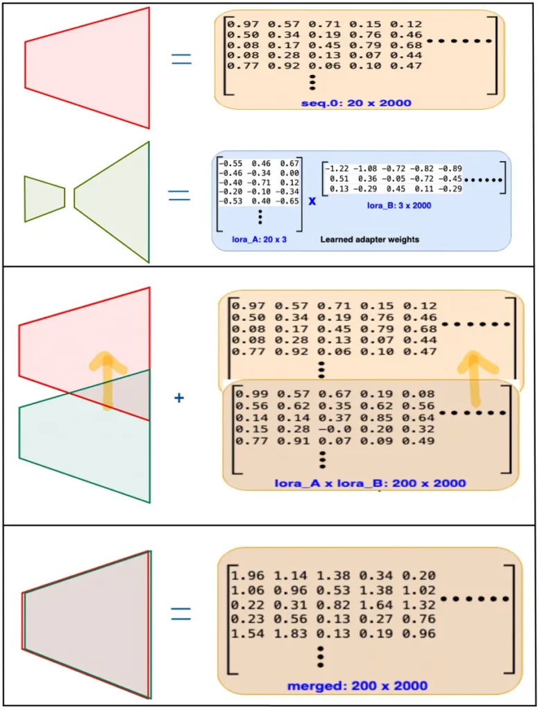
Merging the adapters

While adapter based parameter efficient fine-tuning techniques increase inference latency due to the expanded network size with additional adapter modules, the LoRA adapters are strategically designed to facilitate merging with adoptee matrices when needed, thereby reducing additional inference time. As demonstrated in Part-1 of the blog, the number of parameters upon multiplying both the layers in adapters (seq.0.lora_A x seq.0.lora_B), aligns with the number of parameters in seq.0, and similarly for (seq.2.lora_A x seq.2.lora_B) and seq.2. Leveraging this alignment, element-wise addition can be employed during the merging process, optimizing the inference efficiency of the model.

peft_model_merged_and_unloaded = peft_model.merge_and_unload()
print_trainable_parameters(peft_model_merged_and_unloaded)

Output:
trainable params: 0 || all params: 442602 || trainable%: 0.0

As we can see above, the total number of parameters is back to 442602 and none are trainable. The inference time now, will be same as it was for the base_model.

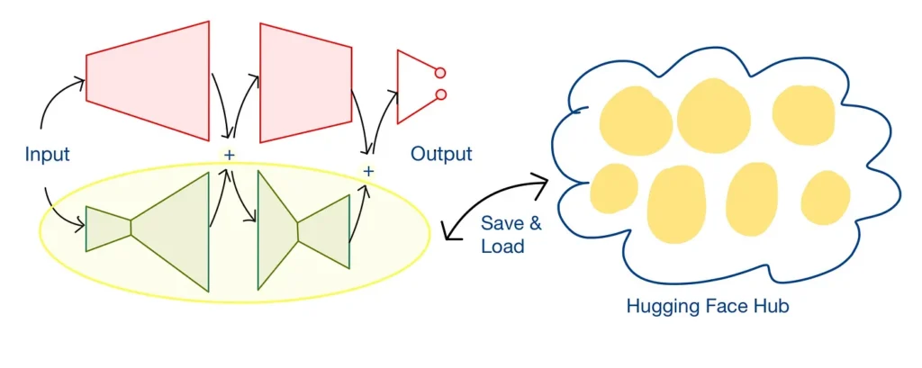
Sharing the model through Hugging Face Hub

It is necessary to have a valid Hugging Face account and you need to have ‘write access token’ to push the model to the hub. You may or may not want to add the token as a git credential. Either ways you will be allowed to login.

Pushing the model to HF Hub

Create a model id and push the peft_model to Hugging Face Hub.

user = "xxx"  # put your user name here
model_name = "peft-lora-with-MLP-model_"
model_id = f"{user}/{model_name}"

peft_model_unmerged.push_to_hub(model_id)

Output:
adapter_model.safetensors: 100% 51.1k/51.1k [00:00<00:00, 110kB/s] CommitInfo(commit_url='https://huggingface.co/s3pi/peft-lora-with-MLP-model_/commit/e395ff324600c273782f66b6900698ca366248ac', commit_message='Upload model', commit_description='', oid='e395ff324600c273782f66b6900698ca366248ac', pr_url=None, pr_revision=None, pr_num=None)

As evident, the adapter size is merely 51 kB. Alternatively, this figure can be derived from the 12,660 parameters, each of 32-bit size, resulting in approximately 51KB (12,660 * 4) Bytes. In contrast, the base model comprises 442,602 parameters, amounting to 1,770KB, a size considerably larger than that of the adapter. This size escalation becomes particularly significant in the context of a large language model.

Loading the model from HF Hub

Now, it only takes one step to load the model from HF Hub. To do this, we can use PeftModel.from_pretrained, passing our pre-trained base model and the model ID:

loaded_model = peft.PeftModel.from_pretrained(base_model_pretrained, model_id)
print_trainable_parameters(f'loaded_model: {loaded_model}')

loaded_model_merged_and_unloaded = loaded_model.merge_and_unload()
print_trainable_parameters(f'merged_model: {merged_model}')

Let’s check if peft_model in our machine and loaded_model from the hub produce the same output:

y_peft = peft_model_merged_and_unloaded(X.to(device))
y_loaded = loaded_model_merged_and_unloaded(X.to(device))
print(torch.allclose(y_peft, y_loaded))

Output:
loaded_model: trainable params: 0 || all params: 455,262 || trainable%: 0.0
merged_model: trainable params: 0 || all params: 442602 || trainable%: 0.0
True

Clean up

Finally, as a clean up step, you may want to delete the repo.

from huggingface_hub import delete_repo
delete_repo(model_id)

Performance

In Section 7 of the LoRA paper¹, it’s demonstrated that low-rank adaptation matrices (adapters) can enhance important features for specific downstream tasks — features that were initially learned but not strongly emphasized in the general pre-training model. They employ a metric called amplification factor to show the same. A higher amplification factor would indicate that the changes in weights of adapter matrix (ΔW) significantly amplify certain features of the original weights of adoptee matrix (W) in the direction of adapter matrix’s (ΔW’s) strongest components, suggesting a more substantial shift in the model’s focus or behavior.

The authors of LoRA demonstrate that a small rank (e.g., r=2) can produce a higher amplification factor than a larger rank (e.g., r=64). This suggests that a few specific directions (or features, in this context, merely 2) in the weight space are essential for adapting the model to a particular task. This insight is particularly useful for efficiently adapting large pre-trained models, such as GPT-3, indicating that modifying a minimal number of directions — and consequently, a limited set of parameters — is sufficient for task-specific adjustments. For various downstream tasks, a unique set of feature directions is likely to be emphasized.

Limitations

• LoRA adapters are notably compact, requiring only a few megabytes of memory, whereas pre-trained models demand several gigabytes. When conducting inference, it is necessary to utilize both the adapters and the pre-trained model. This combination, particularly with today’s large language models, still entails considerable memory usage. To effectively manage these memory requirements during inference, QLoRA emerges as a practical solution involving quantization of parameters.
• An adapter is specifically trained for each sub-task. However, when dealing with a batch containing data for multiple tasks, it is not feasible to load adapters for all these tasks simultaneously.

Additional Remark:
In Figure 1 of the LoRA paper, the parameters initially named A and B are later referred to as B and A, respectively, starting from Section 4 (Method and Implementation). Despite this switch in nomenclature, it’s important to note that both the PEFT implementation and the paper discuss the same parameters. This naming discrepancy is also highlighted in an issue I raised here.

Colab Notebook for further reading: Analyzing LoRA through its Implementation on an MLP.ipynb

Thanks to my colleagues at Sahaj for all the brainstorming sessions.

All images are by the author unless otherwise stated.

[1] Edward J. Hu and Yelong Shen and Phillip Wallis and Zeyuan Allen-Zhu and Yuanzhi Li and Shean Wang and Lu Wang and Weizhu Chen.LoRA: Low-Rank Adaptation of Large Language Models, 2021.

[2] Peft Github

[3] Dive Into LoRA Adapters